Plotting functions may not work as expected during this time.

Map Level Plots
Convection Map Map Time-SeriesFITACF Level Plots
Fan Ball & Stick Summary Plot Range-Time FITACF Time-Series FITACF Time-Series GateRAWACF Level Plots
ACFs Pwr0 StatisticsInformation Plots
Field-of-viewSee plot types tab below for examples
Your plot is being produced, this may take several minutes.
Please do not refresh the page.
This tool is currently using pyDARN v4.3 ![]()
pyDARN is an open source python library for data visualization of SuperDARN data. The source code can be found on the pyDARN github page, with installation instructions found in the pyDARN documentation.
To use pyDARN Online, select the type of plot from the drop down list above, and fill in the form to produce your required plot. It may take up to 2 minutes to produce and display a plot with 24 hours of data, for this reason, the largest epoch for FITACF data allowed to be plotted online is 48 hours and 24 hours in a single calendar day for Map level data. The plots produced on this site are not suitable for publication. Examples of each plot type and a description of the variables presented can be found below.
See below for more information.
Information
Click to buttons below to expand information boxes.
Data and Plot Availability
SuperDARN Canada produces data files as we get them, and as such pyDARN online may not display plots where data was taken in the past few days. Please see our citations policy below or our Data Products page for more information on how to cite SuperDARN data and software.
The FITACF 3.0 files available for use in pyDARN Online use the default options of the RST version 5.0 make_fit command, with the option -fitacf-version 3.0. Map files are produced by the default commands of RST using FITACF 3.0, recent Map files may still be awaiting data from some radars.
You can check our inventory of data by using the ' Check Inventory' button. A calendar of the chosen month and radar will be shown, days which have full data coverage are shown in dark blue, days with partial data coverage are shown in pale blue. If a date has been block listed, the day will not be coloured in. If you require data which has been block listed, you can contact the PI of the radar to get more infomation about why that day might be block listed.
Pre-made 24 hr (00:00-23:59) summary plots are available here to browse. Some radars allow for real-time data streaming, if you are looking for the current radar activity, see the real time fan plots and real time range-time plots.
Parameter Descriptions
| Required Parameter Name | Description | Example Useage |
|---|---|---|
| Start Date and Time | The start date and time of the interval of interest, enter the date as yyyy-mm-dd or choose from the pop up calendar. Choose the time interval from the pop-up time picker, or type in an hour, minute and AM/PM. | Choose from calendar and time picker (browser dependent) |
| End Date and Time | The end date and time of the interval of interest, enter the date as yyyy-mm-dd or choose from the pop up calendar. If you have chosen a start date, the end date will automatically be filled with that date. Choose the time interval from the pop-up time picker, or type in an hour, minute and AM/PM. The end time cannot be more than 48 hours from the start time. | Choose from calendar and time picker (browser dependent) |
| Radar/(s) | Select desired radar from the list of all SuperDARN radars. University of Saskatchewan maintained radars are at the top of the list followed by northern, then southern radars. For a FOV plot, hold down cmd to select multiple radars. | Select from dropdown |
| Beam | SuperDARN radars have varying numbers of beams for each radar. Most have beams numbers from 0-16, 0-22 or 0-24. Be aware that some beams may not have data even if adjacent beams do, it is common for lower numbered beams on radars with 22+ number of beams to be empty of data. This field will automatically update the beam numbers available, so don't forget to reselect the beam if a new radar is chosen. | Select from dropdown |
| Gate | SuperDARN radars have varying numbers of gates in each beam for each radar. Most have gate numbers from 0-74, 0-99 or 0-109. Be aware that some gates may not have data even if adjacent gates do. This field will automatically update the gate numbers available, so don't forget to reselect the gate if a new radar is chosen. | Select from dropdown |
| Parameter | Select the parameter you wish to plot. For Range-Time, Fan and Time-Series Gate plots, you can choose from line-of-sight velocity (ms-1), spectral width (ms-1), power (dB), and elevation (°). For Time-Series plots, you can choose from sky noise (db), transmission frequency (MHz), number of pulsed sequences (Nave), and operation mode (CPID). For ACF plots, the parameter choice is between ACFD or XCFD where available. For Convection Maps you can choose from Fitted, Modelled or Raw velocities, along with the spectral width and power. | Select from dropdown |
| Hemisphere | Choose between the northern and southern hemispheres for convection maps. | Select from dropdown |
| Optional Parameter Name | Description | Example Useage |
| Groundscatter Color (Velocity data only) | If option 'Grey' is chosen, the groundscatter data will appear grey in the velocity data only for Summary plots, Range-Time plots and Fan plots. If 'Not Grey' is chosen, the underlying groundscatter data can be seen. The default is to have the groundscatter greyed out only in the velocity data. | Select from dropdown |
| Groundscatter | If option 'Remove' is chosen, the groundscatter data will be removed for Summary plots, Range-Time plots and Fan plots. The default is to have the groundscatter included. | Select from dropdown |
| Ionospheric scatter | If option 'Remove' is chosen, the ionospheric scatter data will be removed for Summary plots, Range-Time plots and Fan plots. The default is to have the ionospheric scatter included. | Select from dropdown |
| Channel | Data may be recorded on different channels depending on the CPID. Most radars use channel a(0) to record common time data, but can use b(1), c(2) and d(3) for other frequencies and CPIDs at the same time or consecutively in discretionary or special times. The default is to plot all channels, however this may result in two channels of data overplotting each other. If this occurs you can separate them out using this selection. All four channels are available in the dropdown, but it is unlikely that all four channels are utilized at the same time. | Select from dropdown |
| Y-Axis Units/ Range Estimation | Select required units from either Slant Range in kilometers, Ground Scatter Mapped Range in kilometers, or Range Gates. The default is Range Gates for Range-Time and Time-Series plots. The Range Gate option is not available for Fan plots, so the default there is Slant Range. | Select from dropdown |
| Coordinates | Requires a range estimation in distance. Select a latitude or longitude in a coordinate system to plot a range time or summary plot with the coordinates on the y-axis. IT IS THE REPOSNSIBILITY OF THE USER TO ESTABLISH IF THE IS CORRECT PRESENTATION FOR THE DATA. For example, a northernly pointing radar such as Rankin Inlet has very unhelpful data when plotted in longitude, and as the data goes up and over the pole, the plot will only plot the upwards data unless you change the Coord Direction parameter. | Select from dropdown |
| Coord Direction | When plotting using the Coords parameter above in latitudes, you can use this field to see both the 'poleward' data and 'equatorward 'data without them overplotting. Again, it is the responsibility of the user to interpret this data effectively! | Select from dropdown |
| Velocity Range | Select required range from the dropdown. The default setting is -200 to 200 m/s but this may not be large enough to see some structures. | Select from dropdown |
| SNR Range | Select required range from the dropdown. The default value is 0 to 50 dB, however this may be too large or too small to see some structures. | Select from dropdown |
| Spectral Width Range | Select required range from the dropdown. The default value is 0-250 m/s, however this may be too small or too large to see some structures. | Select from dropdown |
| Elevation Range | Select a range from the dropdown. The default value is 0-50 degrees, however this may be too small or too large to see some structures. | Select from dropdown |
| Colorbar Max Value | This option allows the user to select the maximum value of the colour bar for the chose parameter in a Range-Time plot. The default for line-of-sight velocity is 200 m/s, for SNR (power) is 50 dB, for spectral width is 250 m/s and for elevation is 50 degrees. The form will accept any positive number. IF a minimum value is not given, the value selected for the velocity will be used as an absolute limit, setting the lower bound as the negative absolute value of the input. | 200, 50, 250, 50 |
| Colorbar Min Value | This option allows the user to select the minimum value of the colour bar for the chose parameter in a Range-Time plot. The default for line-of-sight velocity is -200 m/s, for SNR (power) is 0 dB, for spectral width is 0 m/s and for elevation is 0 degrees. The form will accept any positive or negative number. If a maximum value is not given, the value selected for the velocity will be used as an absolute limit, setting the upper bound as the positive absolute value of the input. | -200, 0 ,0 ,0 |
| Range Max | This option allows the user to select the maximum value of the range estimation used in a Range-Time plot. Make sure the values entered make sense with the selection of range estimation method. The default is 75 range gates for most radars, or the corresponding slant range, GSMR distance that range gate 75 is located at. | 75 |
| Range Min | This option allows the user to select the minimum value of the range estimation used in a Range-Time plot. Make sure the values entered make sense with the selection of range estimation method. The default is 0 range gates, or the corresponding slant range, GSMR distance that range gate 0 is located at. | 0 |
| Lowest Latitude | For polar plotting, gives the lowest value for plotting on the radial axis (latitude). Default is 30. For Southern hemisphere plots, positive or negative values can be accepted, but will be set to a negative value. | 50 |
| Max Range Gate | When plotting a fan plot, this value will be the furthest range gate you wish to plot, default is 75. | 100 (if range gates extend to this value) |
| Grid Lines | When plotting a fan plot, you can choose to plot with or without the outlines of the individual range gates. | Select from dropdown |
| Plot Blanked Lags | For ACF plots, you can choose to ignore the blanked lag values by setting this option to Do Not Plot Blanked Lags. | Select from dropdown |
| Minimum Freq (kHz) | For pwr0 statistics plots, you can choose to only plot statistics of pwr0 above a given frequency. | 11000 |
| Maximum Freq (kHz) | For pwr0 statistics plots, you can choose to only plot statistics of pwr0 below a given frequency. | 12000 |
| Split Freq (kHz) | For pwr0 statistics plots, you can choose to separate the statistics into two plots, split at the given frequency. | 10000 |
| Statistical Method | For pwr0 statistics plots, you can choose to plot the mean, median or standard deviation . | Select from dropdown |
| Filled Contours | Choose between the default of line-only contours or fill the contours using a red-blue colour map. | Select from dropdown |
| TDiff Correction | TDiff Correction recalculates the elevation angle given the new tdiff value entered. This algorithm uses the method in Shepherd, 2017. | Enter number value. I.E. 0.01 |
| Plot Center | Moves the center of the plot to these coordinates, if left blank the corresponding magnetic or geographic pole is used. | Enter two numbers separated by a comma (lon,lat). E.g. 100, 75 in degrees |
| Plot Extent | Choose how much of the Earth you want to see around the central position of the plot. | Enter two numbers separated by a comma (width, height). E.g. 45, 25 in percentage |
| Plot Tight | Plot zoomed in around the FOV of the radar. Default off. | Select from dropdown. |
Plot Types
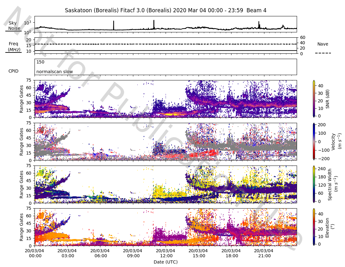
Summary Plots
The plots show signal to noise ratio (dB), velocity (ms-1), spectral width (ms-1), and elevation (°) with respect to the range gate number, or slant range, and date. In addition, sky noise (dB), operating frequency of the radar (MHz), number of pulsed sequences transmitted (Nave), and the mode of operation (CPID) are shown in the first three panels. The figure below shows an example plot of beam 4 of the Saskatoon radar operating on March 4th 2020.
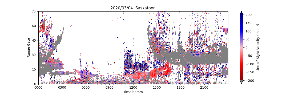
Range-Time Plots
Range-time parameter plots (also known as range-time intensity (RTI) plots) are time series of a radar-measured parameter at range gates 0-75 along a specific beam. Currently pyDARN online supports plotting line-of-sight velocity (ms-1), spectral width (ms-1), power (dB), and elevation (°). The data cam be plotted with either slant range or range gates along the y-axis. The figure below shows an example plot of velocity for beam 4 of the Saskatoon radar operating on March 4th 2020
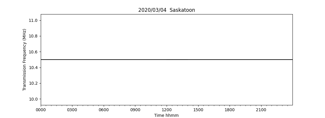
Time-Series Plots
This plot selection will allow you to plot any of the scalar parameters for a selected beam. The parameters include sky noise (db), transmission frequency (MHz), number of pulsed sequences (Nave), and operation mode (CPID).The figure below shows an example plot of transmission frequency for beam 4 of the Saskatoon radar operating on March 4th 2020
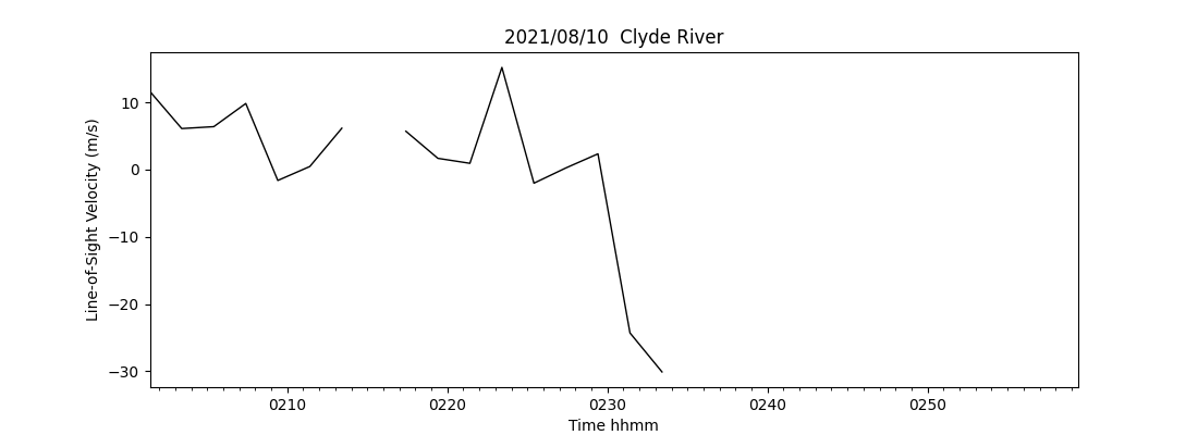
Time-Series Gate Plots
This plot selection will allow you to plot any of the vector parameters for a selected beam in a specified gate. The parameters include line-of-sight velocity (ms-1), spectral width (ms-1), power (dB), and elevation (°).The figure below shows an example plot of line of sight velocity for beam 8, gate 30 for the Clyde River radar operating on 10th August 2021 (channel a). Note that there may be gaps in the plot where no data was recorded for the specified gate, some plots may come back completely blank.
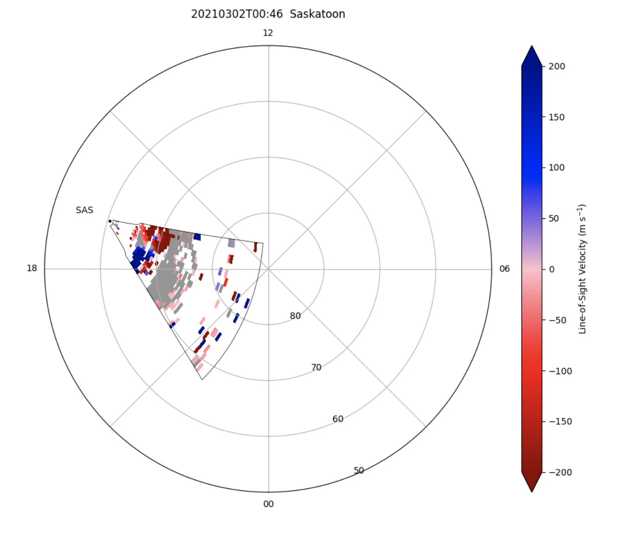
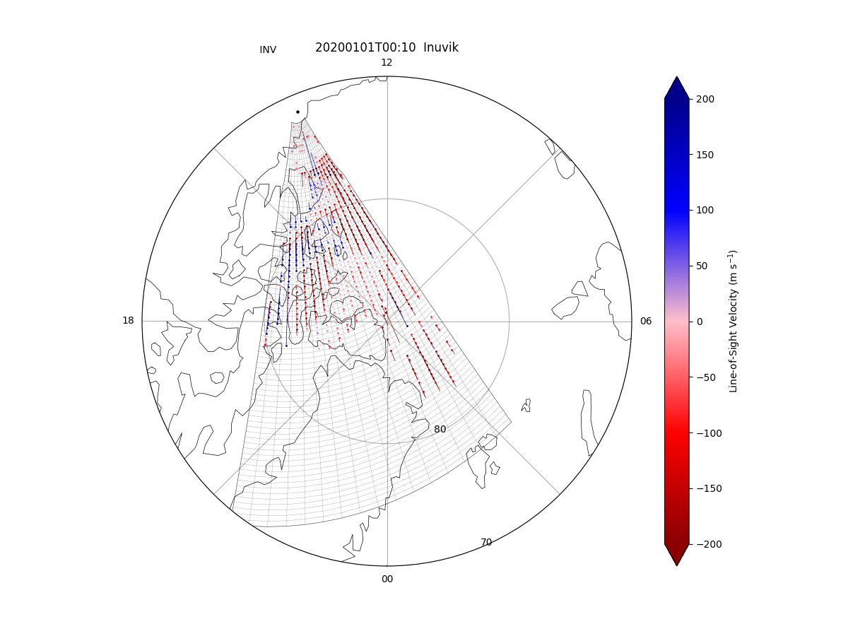
Fan Plots
This plot selection will allow you to plot vector parameters for a selected time for all beams in a fan plot. The parameters include signal to noise ratio (dB), velocity (ms-1), spectral width (ms-1), and elevation (°).The figure below shows an example plot of line-of-sight velocity at Saskatoon radar on March 2nd 2021 at 10:46 AM
ACF Plots
This plot option allows you to plot the Auto-Correlation Function (ACF) of the imaginary and real parts of selected RAWACF data. The example below shows the ACF for the Longyearbyen radar on 6th April 2018.

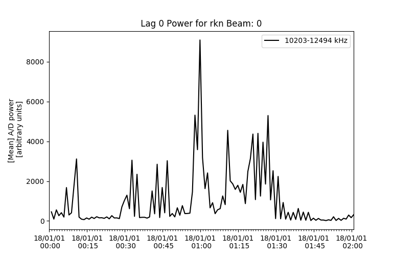
pwr0 Statistics Plots
This plot will calculate and plot a statistic of the lag-0 power of each record as a function of time. This plot option will plot all of a two hour file. The example below shows the mean of the lag0 power for Rankin Inlet on 1st Jan 2018. The second example shows the lag 0 power mean for Longyearbyen, split at 10000 kHz.

Convection Maps
This plot produces a convection map for the given time and hemisphere. The example below shows a convection map on 10th March 2015, using fitted velocity vectors.

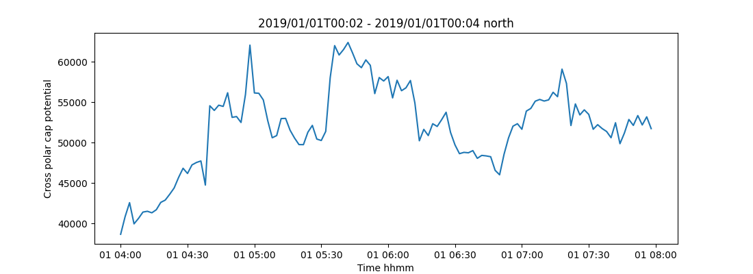
Time Series of Map Data
This plot produces time-series for the given times and hemisphere. The example below shows a time series of map data on 1st January 2024.
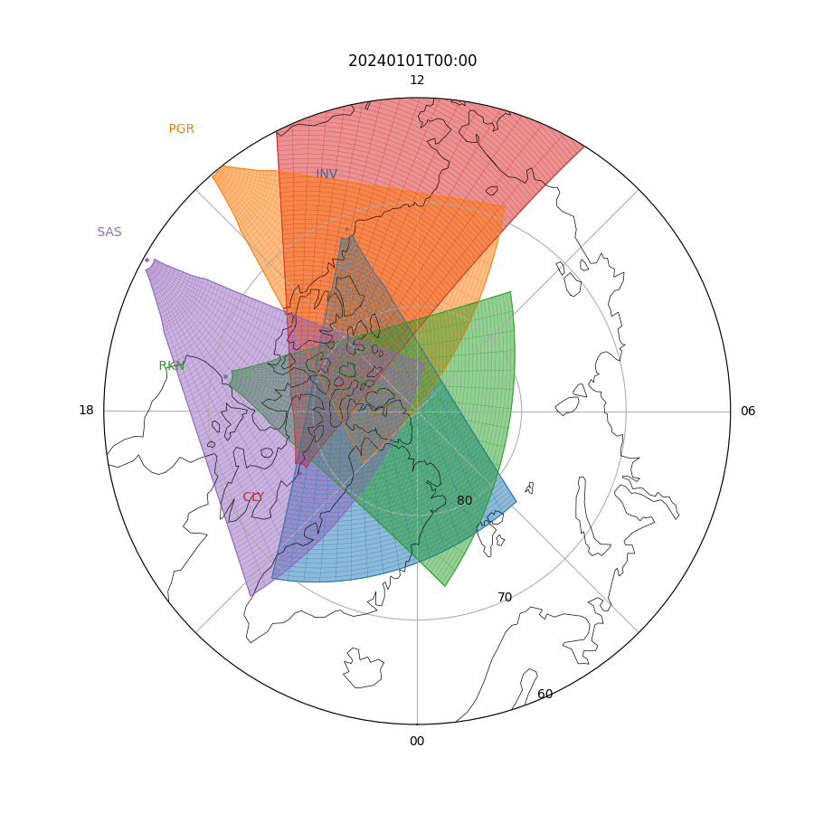
Field of View Plots
This plot produces FOV for the given time and radars. The example below shows SuperDARN Canada's five radars on 1st January 2024.
Ball and Stick Plots
This plot selection will allow you to plot vector parameters for a selected time for all beams in a fan plot with a ball-and-stick appearance. The parameters include signal to noise ratio (dB), velocity (ms-1), spectral width (ms-1), and elevation (°).The figure below shows an example plot of line-of-sight velocity at Saskatoon radar on January 1st 2020.
How To Acknowledge SuperDARN Data
Any publications using SuperDARN Data must include the following text in their acknowledgements:
"The authors acknowledge the use of SuperDARN data. SuperDARN is a collection of radars funded by national scientific funding agencies of Australia, Canada, China, France, Italy, Japan, Norway, South Africa, United Kingdom and the United States of America."
During your study, if using data from individual radars only, please contact the Principal Investigator (PI) of that radar about potential co-authorship. A list of radars, institutions, and their PI's information can be found here.
For SuperDARN Canada managed radars (Saskatoon, Rankin Inlet, Inuvik, Clyde River, and Prince George), contact Dr. Glenn Hussey of the University of Saskatchewan.
SuperDARN is in the process of placing DOI's on their data set. In the meantime, please use any local available services, such as zenodo or FRDR, to DOI your data set.
How To Cite SuperDARN Data
SuperDARN is a made up of 36 radars and 20 institutions, to cite SuperDARN generally, the following reference can be used:
Greenwald, R.A., Baker, K.B., Dudeney, J.R. et al. Space Sci Rev (1995) 71: 761. doi:10.1007/BF00751350
For the general achievements of the SuperDARN Network, the following papers and references within can be used:
Chisham, G., Lester, M., Milan, S.E. et al. A decade of the Super Dual Auroral Radar Network (SuperDARN): scientific achievements, new techniques and future directions. Surv Geophys 28, 33–109 (2007) doi:10.1007/s10712-007-9017-8
Nishitani, N., Ruohoniemi, J.M., Lester, M. et al. Review of the accomplishments of mid-latitude Super Dual Auroral Radar Network (SuperDARN) HF radars. Prog Earth Planet Sci 6, 27 (2019) doi:10.1186/s40645-019-0270-5
* For access to block listed files, please speak to the PI of the radar of interest.